Amortized posterior inference on Gaussian example

Note, you can find the original version of this notebook at https://github.com/sbi-dev/sbi/blob/main/tutorials/01_gaussian_amortized.ipynb in the sbi repository.

In this tutorial, we introduce amortization that is the capability to evaluate the posterior for different observations without having to re-run inference.

We will demonstrate how sbi can infer an amortized posterior for the illustrative linear Gaussian example introduced in Getting Started, that takes in 3 parameters (\(\theta\)).

import torch

from sbi import analysis as analysis
from sbi import utils as utils
from sbi.inference import SNPE, simulate_for_sbi
from sbi.utils.user_input_checks import (
    check_sbi_inputs,
    process_prior,
    process_simulator,
)

Defining simulator, prior, and running inference

Our simulator (model) takes in 3 parameters (\(\theta\)) and outputs simulations of the same dimensionality. It adds 1.0 and some Gaussian noise to the parameter set. For each dimension of \(\theta\), we consider a uniform prior between [-2,2].

num_dim = 3
prior = utils.BoxUniform(low=-2 * torch.ones(num_dim), high=2 * torch.ones(num_dim))

def simulator(theta):
    # linear gaussian
    return theta + 1.0 + torch.randn_like(theta) * 0.1

# Check prior, simulator, consistency
prior, num_parameters, prior_returns_numpy = process_prior(prior)
simulator = process_simulator(simulator, prior, prior_returns_numpy)
check_sbi_inputs(simulator, prior)

# Create inference object. Here, NPE is used.
inference = SNPE(prior=prior)

# generate simulations and pass to the inference object
theta, x = simulate_for_sbi(simulator, proposal=prior, num_simulations=2000)
inference = inference.append_simulations(theta, x)

# train the density estimator and build the posterior
density_estimator = inference.train()
posterior = inference.build_posterior(density_estimator)

Running 2000 simulations.:   0%|          | 0/2000 [00:00<?, ?it/s]


 Neural network successfully converged after 70 epochs.

Amortized inference

Note that we have not yet provided an observation to the inference procedure. In fact, we can evaluate the posterior for different observations without having to re-run inference. This is called amortization. An amortized posterior is one that is not focused on any particular observation. Naturally, if the diversity of observations is large, any of the inference methods will need to run a sufficient number of simulations for the resulting posterior to perform well across these diverse observations.

Let’s say we have not just one but two observations \(x_{obs~1}\) and \(x_{obs~2}\) for which we aim to do parameter inference.

Note: For real observations, of course, you would not have access to the ground truth \(\theta\).

# generate the first observation
theta_1 = prior.sample((1,))
x_obs_1 = simulator(theta_1)
# now generate a second observation
theta_2 = prior.sample((1,))
x_obs_2 = simulator(theta_2)

We can draw samples from the posterior given \(x_{obs~1}\) and then plot them:

posterior_samples_1 = posterior.sample((10000,), x=x_obs_1)

# plot posterior samples
_ = analysis.pairplot(
    posterior_samples_1, limits=[[-2, 2], [-2, 2], [-2, 2]], figsize=(5, 5),
    labels=[r"$\theta_1$", r"$\theta_2$", r"$\theta_3$"],
    points=theta_1 # add ground truth thetas
)

Drawing 10000 posterior samples:   0%|          | 0/10000 [00:00<?, ?it/s]

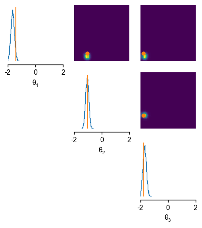
The inferred distirbutions over the parameters given the first observation \(x_{obs~1}\) match the parameters \(\theta_{1}\) (shown in orange), we used to generate our first observation \(x_{obs~1}\).

Since the learned posterior is amortized, we can also draw samples from the posterior given the second observation \(x_{obs~2}\) without having to re-run inference:

posterior_samples_2 = posterior.sample((10000,), x=x_obs_2)

# plot posterior samples
_ = analysis.pairplot(
    posterior_samples_2, limits=[[-2, 2], [-2, 2], [-2, 2]], figsize=(5, 5),
    labels=[r"$\theta_1$", r"$\theta_2$", r"$\theta_3$"],
    points=theta_2 # add ground truth thetas
)

Drawing 10000 posterior samples:   0%|          | 0/10000 [00:00<?, ?it/s]

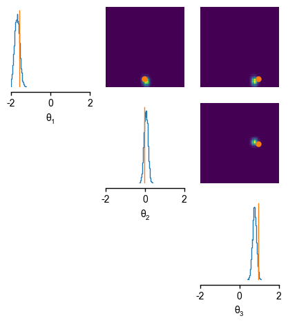
The inferred distirbutions over the parameters given the second observation \(x_{obs~2}\) also match the ground truth parameters \(\theta_{2}\) we used to generate our second test observation \(x_{obs~2}\).

This in a nutshell demonstrates the benefit of amortized methods.

Next steps

Now that you got familiar with amortization, we recommend checking out inferring parameters for a single observation which introduces the concept of multi round inference for a single observation to be more sampling efficient.