The flexible interface

In the previous tutorial, we have demonstrated how sbi can be used to run simulation-based inference with just a single line of code.

In addition to this simple interface, sbi also provides a flexible interface which provides several additional features implemented in sbi.

Note, you can find the original version of this notebook at https://github.com/sbi-dev/sbi/blob/main/tutorials/02_flexible_interface.ipynb in the sbi repository.

Features

The flexible interface offers the following features (and many more):

• performing sequential posterior estimation by focusing on a particular observation over multiple rounds. This can decrease the number of simulations one has to run, but the inference procedure is no longer amortized (tutorial).
• specify your own density estimator, or change hyperparameters of existing ones (e.g. number of hidden units for NSF) (tutorial).
• use an embedding_net to learn summary features from high-dimensional simulation outputs (tutorial).
• provide presimulated data
• choose between different methods to sample from the posterior.
• use calibration kernels as proposed by Lueckmann, Goncalves et al. 2017.

Main syntax

from sbi.utils.user_input_checks import process_prior, process_simulator, check_sbi_inputs
from sbi.inference import SNPE, simulate_for_sbi

prior, num_parameters, prior_returns_numpy = process_prior(prior)
simulator = process_simulator(simulator, prior, prior_returns_numpy)
check_sbi_inputs(simulator, prior)
inference = SNPE(prior)

theta, x = simulate_for_sbi(simulator, proposal=prior, num_simulations=1000)
density_estimator = inference.append_simulations(theta, x).train()
posterior = inference.build_posterior(density_estimator)

Linear Gaussian example

We will show an example of how we can use the flexible interface to infer the posterior for an example with a Gaussian likelihood (same example as before). First, we import the inference method we want to use (SNPE, SNLE, or SNRE) and other helper functions.

import torch

from sbi import analysis as analysis
from sbi import utils as utils
from sbi.inference import SNPE, simulate_for_sbi
from sbi.utils.user_input_checks import (
    check_sbi_inputs,
    process_prior,
    process_simulator,
)

Next, we define the prior and simulator:

num_dim = 3
prior = utils.BoxUniform(low=-2 * torch.ones(num_dim), high=2 * torch.ones(num_dim))

def linear_gaussian(theta):
    return theta + 1.0 + torch.randn_like(theta) * 0.1

In the flexible interface, you have to ensure that your simulator and prior adhere to the requirements of sbi. You can do so with the process_simulator() and process_prior() functions, which prepare them appropriately. Finally, you can call check_sbi_input() to make sure they are consistent which each other.

# Check prior, return PyTorch prior.
prior, num_parameters, prior_returns_numpy = process_prior(prior)

# Check simulator, returns PyTorch simulator able to simulate batches.
simulator = process_simulator(linear_gaussian, prior, prior_returns_numpy)

# Consistency check after making ready for sbi.
check_sbi_inputs(simulator, prior)

Then, we instantiate the inference object:

inference = SNPE(prior=prior)

Next, we run simulations. You can do so either by yourself by sampling from the prior and running the simulator (e.g. on a compute cluster), or you can use a helper function provided by sbi called simulate_for_sbi. This function allows to parallelize your code with joblib.

theta, x = simulate_for_sbi(simulator, proposal=prior, num_simulations=2000)

Running 2000 simulations.:   0%|          | 0/2000 [00:00<?, ?it/s]

We then pass the simulated data to the inference object. theta and x should both be a torch.Tensor of type float32.

inference = inference.append_simulations(theta, x)

Next, we train the neural density estimator.

density_estimator = inference.train()

 Neural network successfully converged after 70 epochs.

Lastly, we can use this density estimator to build the posterior:

posterior = inference.build_posterior(density_estimator)

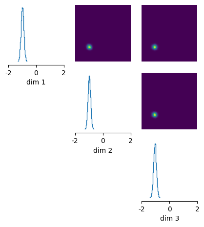
Once we have obtained the posterior, we can .sample(), .log_prob(), or .pairplot() in the same way as for the simple interface.

x_o = torch.zeros(3,)

posterior_samples = posterior.sample((10000,), x=x_o)

# plot posterior samples
_ = analysis.pairplot(
    posterior_samples, limits=[[-2, 2], [-2, 2], [-2, 2]], figsize=(5, 5)
)

Drawing 10000 posterior samples:   0%|          | 0/10000 [00:00<?, ?it/s]

We can always print the posterior to know how it was trained:

print(posterior)

Posterior conditional density p(θ|x) of type DirectPosterior. It samples the posterior network and rejects samples that
            lie outside of the prior bounds.