Multi-round inference

In the previous tutorials, we have inferred the posterior using single-round inference. In single-round inference, we draw parameters from the prior, simulate the corresponding data, and then train a neural network to obtain the posterior. However, if one is interested in only one particular observation x_o sampling from the prior can be inefficient in the number of simulations because one is effectively learning a posterior estimate for all observations in the prior space. In this tutorial, we show how one can alleviate this issue by performing multi-round inference with sbi.

Multi-round inference also starts by drawing parameters from the prior, simulating them, and training a neural network to estimate the posterior distribution. Afterwards, however, it continues inference in multiple rounds, focusing on a particular observation x_o. In each new round of inference, it draws samples from the obtained posterior distribution conditioned at x_o (instead of from the prior), simulates these, and trains the network again. This process can be repeated arbitrarily often to get increasingly good approximations to the true posterior distribution at x_o.

Running multi-round inference can be more efficient in the number of simulations, but it will lead to the posterior no longer being amortized (i.e. it will be accurate only for a specific observation x_o, not for any x).

Note, you can find the original version of this notebook at https://github.com/sbi-dev/sbi/blob/main/tutorials/03_multiround_inference.ipynb in the sbi repository.

Main syntax

import torch

from sbi.analysis import pairplot
from sbi.inference import SNPE, simulate_for_sbi
from sbi.utils import BoxUniform
from sbi.utils.user_input_checks import (
    check_sbi_inputs,
    process_prior,
    process_simulator,
)

# 2 rounds: first round simulates from the prior, second round simulates parameter set
# that were sampled from the obtained posterior.
num_rounds = 2
num_dim = 3
# The specific observation we want to focus the inference on.
x_o = torch.zeros(num_dim,)
prior = BoxUniform(low=-2 * torch.ones(num_dim), high=2 * torch.ones(num_dim))
simulator = lambda theta: theta + torch.randn_like(theta) * 0.1

# Ensure compliance with sbi's requirements.
prior, num_parameters, prior_returns_numpy = process_prior(prior)
simulator = process_simulator(simulator, prior, prior_returns_numpy)
check_sbi_inputs(simulator, prior)

inference = SNPE(prior)

posteriors = []
proposal = prior

for _ in range(num_rounds):
    theta, x = simulate_for_sbi(simulator, proposal, num_simulations=500)

    # In `SNLE` and `SNRE`, you should not pass the `proposal` to
    # `.append_simulations()`
    density_estimator = inference.append_simulations(
        theta, x, proposal=proposal
    ).train()
    posterior = inference.build_posterior(density_estimator)
    posteriors.append(posterior)
    proposal = posterior.set_default_x(x_o)

Running 500 simulations.:   0%|          | 0/500 [00:00<?, ?it/s]


 Neural network successfully converged after 105 epochs.


Drawing 500 posterior samples:   0%|          | 0/500 [00:00<?, ?it/s]



Running 500 simulations.:   0%|          | 0/500 [00:00<?, ?it/s]


Using SNPE-C with atomic loss
 Neural network successfully converged after 36 epochs.

Linear Gaussian example

Below, we give a full example of inferring the posterior distribution over multiple rounds.

First, we define a simple prior and simulator and ensure that they comply with sbi by using process_simulator(), process_prior() and check_sbi_inputs():

def linear_gaussian(theta):
    return theta + 1.0 + torch.randn_like(theta) * 0.1

# Check prior, return PyTorch prior.
prior, num_parameters, prior_returns_numpy = process_prior(prior)

# Check simulator, returns PyTorch simulator able to simulate batches.
simulator = process_simulator(linear_gaussian, prior, prior_returns_numpy)

# Consistency check after making ready for sbi.
check_sbi_inputs(simulator, prior)

Then, we instantiate the inference object:

inference = SNPE(prior=prior)

And we can run inference. In this example, we will run inference over 2 rounds, potentially leading to a more focused posterior around the observation x_o.

num_rounds = 2
x_o = torch.zeros(
    3,
)

posteriors = []
proposal = prior

for _ in range(num_rounds):
    theta, x = simulate_for_sbi(simulator, proposal, num_simulations=500)
    density_estimator = inference.append_simulations(
        theta, x, proposal=proposal
    ).train()
    posterior = inference.build_posterior(density_estimator)
    posteriors.append(posterior)
    proposal = posterior.set_default_x(x_o)

Running 500 simulations.:   0%|          | 0/500 [00:00<?, ?it/s]


 Neural network successfully converged after 58 epochs.


Drawing 500 posterior samples:   0%|          | 0/500 [00:00<?, ?it/s]



Running 500 simulations.:   0%|          | 0/500 [00:00<?, ?it/s]


Using SNPE-C with atomic loss
 Neural network successfully converged after 28 epochs.

Note that, for num_rounds>1, the posterior is no longer amortized: it will give good results when sampled around x=observation, but possibly bad results for other x.

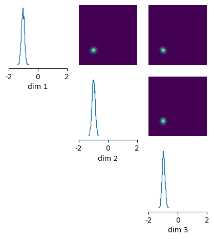
Once we have obtained the posterior, we can .sample(), .log_prob(), or .pairplot() in the same way as for the simple interface.

posterior_samples = posterior.sample((10000,), x=x_o)

# plot posterior samples
fig, ax = pairplot(
    posterior_samples, limits=[[-2, 2], [-2, 2], [-2, 2]], figsize=(5, 5)
)

Drawing 10000 posterior samples:   0%|          | 0/10000 [00:00<?, ?it/s]