Getting started with sbi

Note, you can find the original version of this notebook at https://github.com/sbi-dev/sbi/blob/main/tutorials/00_getting_started_flexible.ipynb in the sbi repository.

sbi provides a simple interface to run state-of-the-art algorithms for simulation-based inference.

The overall goal of simulation-based inference is to algorithmically identify model parameters which are consistent with data.

In this tutorial we demonstrate how to get started with the sbi toolbox and how to perform parameter inference on a simple model.

Each of the implemented inference methods takes three inputs: 1. observational data (or summary statistics thereof) - the observations 1. a candidate (mechanistic) model - the simulator 1. prior knowledge or constraints on model parameters - the prior

If you are new to simulation-based inference, please first read the information in the tutorial README or the website to familiarise with the motivation and relevant terms.

import torch

from sbi import analysis as analysis
from sbi import utils as utils
from sbi.inference import SNPE, simulate_for_sbi
from sbi.utils.user_input_checks import (
    check_sbi_inputs,
    process_prior,
    process_simulator,
)

Parameter inference in a linear Gaussian example

For this illustrative example, we consider a model simulator, that takes in 3 parameters (\(\theta\)). For simplicity, the simulator outputs simulations of the same dimensionality and adds 1.0 and some Gaussian noise to the parameter set.

Note: This is where you instead would use your specific simulator with its parameters.

For the 3-dimensional parameter space we consider a uniform prior between [-2,2].

Note: This is where you would incorporate prior knowlegde about the parameters you want to infer, e.g., ranges known from literature.

num_dim = 3
prior = utils.BoxUniform(low=-2 * torch.ones(num_dim), high=2 * torch.ones(num_dim))

def simulator(theta):
    # linear gaussian
    return theta + 1.0 + torch.randn_like(theta) * 0.1

We have to ensure that your simulator and prior adhere to the requirements of sbi such as returning torch.Tensors in a standardised shape.

You can do so with the process_simulator() and process_prior() functions, which prepare them appropriately. Finally, you can call check_sbi_input() to make sure they are consistent which each other.

# Check prior, return PyTorch prior.
prior, num_parameters, prior_returns_numpy = process_prior(prior)

# Check simulator, returns PyTorch simulator able to simulate batches.
simulator = process_simulator(simulator, prior, prior_returns_numpy)

# Consistency check after making ready for sbi.
check_sbi_inputs(simulator, prior)

Next, we instantiate the inference object. Here, to neural perform posterior estimation (NPE):

Note: Single round sequential NPE which we call via SNPE corresponds to NPE.

Note: This is where you could specify an alternative inference object such as (S)NRE for ratio estimation or (S)NLE for likelihood estimation. Here, you can see all implemented methods.

inference = SNPE(prior=prior)

Next, we need simulations, or more specifically, pairs of parameters \(\theta\) which we sample from the prior and corresponding simulations \(x = \mathrm{simulator} (\theta)\). The sbi helper function called simulate_for_sbi allows to parallelize your code with joblib.

Note: If you already have your own parameters, simulation pairs which were generated elsewhere (e.g., on a compute cluster), you would add them here.

theta, x = simulate_for_sbi(simulator, proposal=prior, num_simulations=2000)

Running 2000 simulations.:   0%|          | 0/2000 [00:00<?, ?it/s]

We then pass the simulated data to the inference object. Both theta and x should be a torch.Tensor of type float32.

inference = inference.append_simulations(theta, x)

Next, we train the neural density estimator to learn the association between the simulated data (or data features) and the underlying parameters:

density_estimator = inference.train()

 Neural network successfully converged after 77 epochs.

Finally, we use this density estimator to build the posterior distribution \(p(\theta|x)\), i.e., the distributions over paramters \(\theta\) given observation \(x\).

Effectively, build_posterior acts as a wrapper for the raw density estimator that among other features (which go beyond the scope of this introductory tutorial) allows us to sample parameters \(\theta\) from the posterior via .sample(), i.e., parameters that are likely given the observation \(x\).

We can also get log-probabilities under the posterior via .log_prob(), i.e., we can evaluate the likelihood of parameters \(\theta\) given the observation \(x\).

posterior = inference.build_posterior(density_estimator)

print(posterior) # prints how the posterior was trained

Posterior conditional density p(θ|x) of type DirectPosterior. It samples the posterior network and rejects samples that
            lie outside of the prior bounds.

Visualisations of the inferred posterior for a new observation

Let’s say we have made some observation \(x_{obs}\) for which we now want to infer the posterior:

Note: this is where your experimental observation would come in. For real observations, of course, you would not have access to the ground truth \(\theta\).

theta_true = prior.sample((1,))
# generate our observation
x_obs = simulator(theta_true)

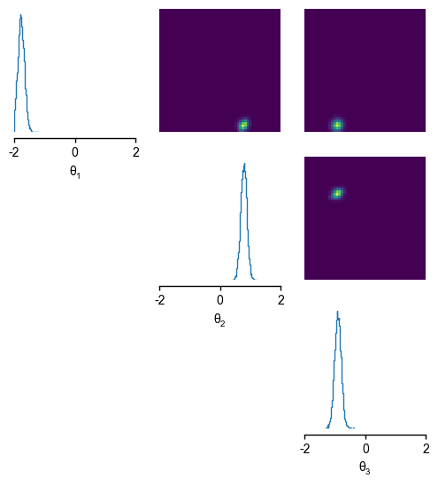
Given this observation, we can sample from the posterior \(p(\theta|x_{obs})\) and visualise the univariate and pairwise marginals for the three parameters via analysis.pairplot().

samples = posterior.sample((10000,), x=x_obs)
_ = analysis.pairplot(samples, limits=[[-2, 2], [-2, 2], [-2, 2]], figsize=(6, 6),labels=[r"$\theta_1$", r"$\theta_2$", r"$\theta_3$"])

Drawing 10000 posterior samples:   0%|          | 0/10000 [00:00<?, ?it/s]

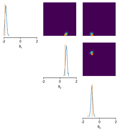
Assessing the posterior for the known \(\theta, x\) - pair

For this special case, we have access to the ground-truth parameters that generated the observation. We can thus assess if the inferred distributions over the parameters match the parameters \(\theta_{true}\) we used to generate our test observation \(x_{obs}\).

samples = posterior.sample((10000,), x=x_obs)
_ = analysis.pairplot(samples, points=theta_true, limits=[[-2, 2], [-2, 2], [-2, 2]], figsize=(6, 6), labels=[r"$\theta_1$", r"$\theta_2$", r"$\theta_3$"])

Drawing 10000 posterior samples:   0%|          | 0/10000 [00:00<?, ?it/s]

The log-probability should ideally indicate that the true parameters, given the corresponding observation, are more likely than a different set of randomly chosen parameters from the prior distribution.

Relative to the obtained log-probabilities, we can investigate the range of log-probabilities of the parameters sampled from the posterior.

# first sample an alternative parameter set from the prior
theta_diff = prior.sample((1,))

log_probability_true_theta = posterior.log_prob(theta_true, x=x_obs)
log_probability_diff_theta = posterior.log_prob(theta_diff, x=x_obs)
log_probability_samples = posterior.log_prob(samples, x=x_obs)

print( r'high for true theta :', log_probability_true_theta)
print( r'low for different theta :', log_probability_diff_theta)
print( r'range of posterior samples: min:', torch.min(log_probability_samples),' max :', torch.max(log_probability_samples))

high for true theta : tensor([2.0030])
low for different theta : tensor([-142.0334])
range of posterior samples: min: tensor(-8.5509)  max : tensor(4.1429)

Next steps

For sbi contributers, we recommend directly heading over to Inferring parameters for multiple observations which introduces the concept of amortization.

For users and sbi beginners, we recommend going through the example for a scientific simulator from neuroscience to see a scientific use case.

Alternatively, also head over to Inferring parameters for multiple observations which introduces the concept of amortization.